The data for the targets come from the Cook Political Report. At some point I will get around to computing these myself. The delegate data is (so far) manually entered.

delegates <- data.frame(State = c("Iowa", "New Hampshire"),
                        Clinton_percentage=c(49.86, 37.95), Sanders_percentage=c(49.57, 60.4),
                        Clinton_target=c(13, 9), Sanders_target=c(31, 15))

We can plot these against each other and see how well we do! I much prefer log-odds ratios to percentages, which require a little bit of an intro.

The more positive the number, the more the state is in support of Clinton and vice versa. 0 is perfectly equal, infinity is 100% Clinton and -infinity is 100% Sanders. A +/-1 is about one standard deviation off, which is 27 or 73%. Regardless of who “won” the state, above the diagonal means Clinton is exceeding expecations, below Sanders is.

plot <- ggplot(delegates, aes(x = log(Clinton_target/Sanders_target), y = log(Clinton_percentage/Sanders_percentage),
                              fill = log(Clinton_target/Sanders_target) - log(Clinton_percentage/Sanders_percentage))) +
  #geom_text( aes(label=State), hjust = 0, vjust = 0 ) +
  geom_point( aes(size = Clinton_target+Sanders_target), shape=21) +
  scale_size_continuous(range = c(2,7), limits = c(14,475)) +
  scale_fill_gradientn(colours = c("blue", "grey", "red"), name="Candidate ahead", limits=c(-2,2)) +
  labs(title = "Targets v Results", x = "Targets", y = "Results", size = "Total delegates") +
  geom_abline(intercept = 0, slope=1, alpha = 0.5) +
  xlim(-1,1) + ylim(-1,1)
plot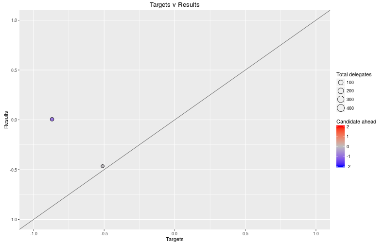

This is interesting since it shows that Sanders is “winning”” (points are y-negative), but it also shows that, at this point, Clinton is meeting or exceeding targets. This disagrees the media narrative, which unfortunately has some influence on future primaries, so we’ll see. Another interesting thing that this might shed some light as to if momentum really exists.

Edit history

• Feb 14: edited language
• Feb 12: changed to ggplot2
• Feb 10: original edit