A recurring them in political science is trying to understand how lawmakers vote. A popular one developed in 1998 by Keith Krehbiel is pivotal politics. Pivotal politics is usually presented as a line graph, but I wanted to see it as a 2d-plot, hence the “revisit”. This is also the first of a few posts on an analysis of a political economics paper, more on that soon!

Basic assumptions

Pivotal politics works on a few key assumptions. First of all, it assumes that there is a one dimensional ranking of legislators on any given issue (note that this means that the ranking might look different on, for example, healthcare and gun control). Secondly, it assumes that lawmakers are “rational actors”, this means that they have an ideal policy point, and that they are trying to reach said point. These assumptions are simplifications of reality, and they fail if we push them to hard, but for now they’ll do.

So what does pivotal politics say? First of all, it aligns all the legislators according to their ideal points. Secondly, it places two points on the line: the status quo s, and the bill b. The legislators’ vote is simply: am I closer to the bill than the status-quo? So much for the theory, it makes sense.

Since the scale is linear, if a legislator supports the bill, then either everyone to one side supports the bill (same for opposition). This is where the power of pivotal politics takes place: the pivots. Our first pivot is the median legislator, m. If m approves the bill, then the bill has at least majority support.

We can plot this! This is a two-input model, so two dimensions: horizontal is bill, vertical is status-quo. Arbitrarily, I’m going to make the values range on the interval [0,1]. Every point corresponds therefore corresponds to a (b, s) pair. Given that pair, we can find who is on the border for supporting it by taking the average. However, the “direction” of the support is still missing, it is established by the sign of b-s, it points away from the status quo. For example, a support of 0.2 means that legislator 0.2 is in favor of it, so is everyone greater than 0.2. A support of -0.2 has the same legislator being the “border”, but everyone smaller than the legislator supports it, failing majority support.

In this plot, we only care about majority support, so it looks rather simple.

precision <- 1000
points <- expand.grid(b = 0:precision/precision, s = 0:precision/precision + 1/(2*precision))
points$support <- sign(points$b-points$s)*(points$b + points$s)/2
points <- mutate(points, majority = (support%%1)<0.5) %>%
  mutate(status = ifelse(majority, "Passes", "Fails"))
ggplot(points, aes(x = b, y = s, fill = status)) +
  geom_raster() +
  labs(x = "Bill", y = "Status Quo", main = "Majority support") +
  scale_fill_manual(values = c("red", "blue")) +
  guides(fill = guide_legend(title="Bill status")) +
  theme(text = element_text(size=20)) + coord_equal()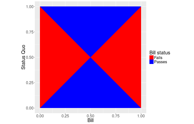

However, many legislatures are more complicated than that: they also have an executive with a veto power, and some (I’m looking at you, Senate), have a filibuster power. We are going to focus on the federal government, since this is what most readers are probably familiar with. The answer to this is simply… more pivots!

The veto power

We are going to start with the veto power, since it is more common. The president, p is added to the line, although it’s not really a pivot (more on that later). If the president opposes the bill, it gets vetoed. On the same side as the president is the veto pivot, v. If v and everyone to the opposite of the president from v opposes the veto (approves the bill), then they can override the veto and enact the bill. If v were on the other side, this would imply v needing the support of a legislator agreeing with the president, which would not make sense.

This is the same plot as above, but with the presidential veto. I’m going to assume a president at -1, where the president is doesn’t change that much. This allows the president to veto anything that has positive support, but the veto will be overturned if it has more than 2/3 support. This means that anything with a support of 1/3 or more will be effectively vetoed.

president <- 0
points <- mutate(points, veto = support>president) %>%
  mutate(veto_overturned = support%%1 < 1/3) %>%
  mutate(label = ifelse(majority,
                        ifelse(veto,
                               ifelse(veto_overturned,
                                      "Passes - Veto overturned",
                                      "Fails - Veto"),
                               "Passes"),
                        "Fails"))
ggplot(points, aes(x = b, y = s, fill = label)) +
  geom_raster() +
  labs(x = "Bill", y = "Status Quo", main = "Majority support") +
  scale_fill_manual(values = c("red", "yellow", "blue", "navy")) +
  guides(fill = guide_legend(title="Bill status")) +
  theme(text = element_text(size=20)) + coord_equal()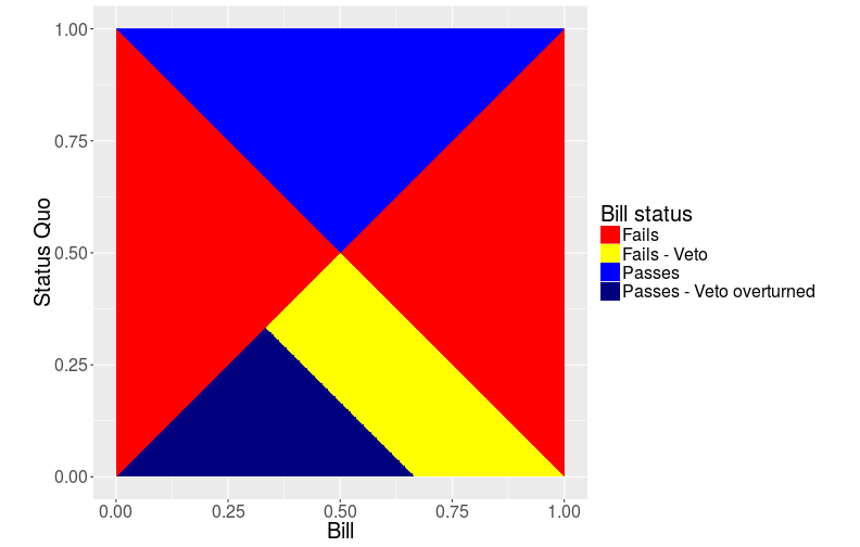

This is where the first interesting result comes up: if the status quo is between 1/3 and 1/2, no bill will ever pass. This can be thought of as the president trying to preserve liked status quos, this is reasonable.

“Let’s keep the debate going! Here’s a cookbook”

Finally, the wonderful filibuster. Filibustering, or the threat thereof, is a technique used to stop a bill from being passed by simply never ending the debate, since stopping the debate requires a super-majority. So we add two filibuster pivots f, one for each side. However, for any particular bill, we only need it on the side of the opposition, since legislators in support of the bill won’t filibuster it.

In generating the plot, I check for filibuster first, since a filibustered bill will not make it to a veto. Similarly, an overturned veto vote can also overcome a filibuster vote, so I do not check for that.

points <- mutate(points, filibuster = support%%1 > 0.4) %>%
    mutate(label = ifelse(majority,
                        ifelse(filibuster,
                               "Fails - Filibustered",
                               ifelse(veto,
                                      ifelse(veto_overturned,
                                             "Passes - Veto overturned",
                                             "Fails - Veto"),
                                      "Passes")),
                        "Fails"))
ggplot(points, aes(x = b, y = s, fill = label)) +
  geom_raster() +
  labs(x = "Bill", y = "Status Quo", main = "Majority support") +
  scale_fill_manual(values = c("red", "orange", "yellow", "blue", "navy")) +
  guides(fill = guide_legend(title="Bill status")) +
  theme(text = element_text(size=20)) + coord_equal()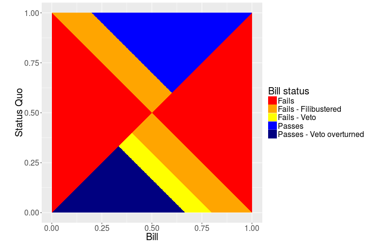

This is even worse: any status quo between 1/3 and 3/5 (0.33 and 0.6) will never be changed. That interval is appropriately named the gridlock interval. Not only that, but most status quos will result in a bill at either the veto or the filibuster pivot, avoiding the median entirely.

Consequences

This has some interesting consequences for real world politics. First of all, moderates are frustrated: they will almost never see one of their ideal bills pass, this is an often-advanced explanation for the polarization of Congress. Secondly, through careful executive orders or other such actions, the president can move the status quo to be at the edge of the gridlock interval, resulting in Congress being unable to do anything. Thirdly, it shows that the president does have some influence on the legislature through the veto power: a president from a different party moves the veto pivot to the other side. Finally, it provides some explanation as to why when republicans took control of Congress (the median pivot), not much actually changed: the pivots are firmly in different parties.

Further research

I am going to stop this introduction here, however a few more posts are in the works! First of all, there is going to be an introduction to DW-NOMINATE, a fantastic tool to actually rank legislators on the scale we’ve been talking about. Using these scores and the fantastic continuing work of its creators, I’m hoping to do some interesting plots of current Congress and their votes. Secondly, there are interesting expansions on pivotal politics and I’m hoping to do some analysis of those as well.

As always, thoughts are welcome!